
Probably the most explored and most favorable use case to explain the power of optimization, hence the need to adapt the mathematical in your organization for increased efficiency of your resources and cost savings.
Problem Description
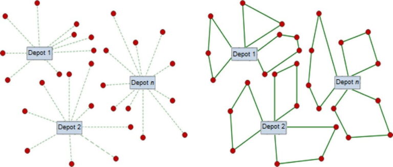
Consider a company having to serve N customers. The company has a central distribution point/s (hub). The company has a fleet of vehicles available at the hub which can carry different types of products and deliver it to the customer locations to fulfill the demand. Now, the company has the information of the demand of each product at each customer location. The planning department with this information, assigns vehicles with the required products to the customer locations. The vehicle then travels to its prescribed location to fulfill the demand.
Simple? Now, consider having to travel hundreds of customer locations with thousands of products to be delivered, and you must fill the vehicle with appropriate products and make a schedule for the vehicle. Now it does not seem so simple. Having we stated the broad problem statement, we shall now move on to discuss some real-world scenarios that can be faced and should be tackled.
Real World Constraints
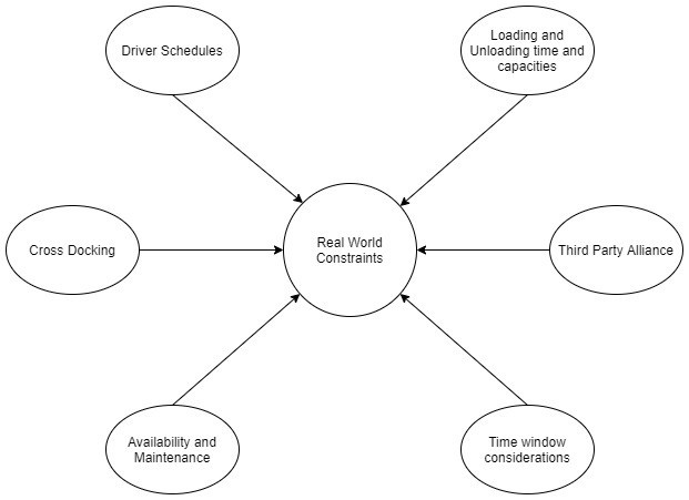
- Minimizing the number of vehicles utilized may not always be the optimization criteria in the day-to-day or even regular scheduling activities. The fleet size is usually determined beforehand. It is the restriction of the driver time that is often the point of concern as the drivers are paid on contractual basis, the route time may exceed the minimum time but less than the maximum time in the contract.
- Driver schedule needs to be considered while developing the routes for the said vehicles while including their break times, curfew hours that might be a policy of the specific region.
- Often, companies face shortfall of fleet and hence resort third party companies to fill in the void or many times completely outsource the same. In these cases, the cost factor play an important role.
- There are cases wherein the company pays only for the first and the last trip, which makes us to plan a linear path rath than a circular one which lead to making a Hamiltonian path that is reaching the farthest point last or first.
- There is a need for delivery within time at select locations to support the concept of inter-tour or cross-docking concepts. This happens when a vehicle delivers to a location from where another scheduled service is to happen. That is another vehicle may pick up the goods from the location which may or may not be under the purview of the model. We must specify time windows for such time bound deliveries.
- The resources for example, unloading cranes, forklift, etc, are limited. The number of vehicles allowed at the location at the same time should be restricted.
- The vehicle availability and maintenance activities should be considered.
- Reverse Logistics based on the business needs can also be introduced
Dynamic nature of the vehicle routing problem makes it even more interesting and complex problem to target.
Apart from these, there can be many more such real-world problems that needs to be accommodated in the model o make the solution realistic and as close to implementation as possible.
Sample problem using PuLP
We shall now have a look at a sample problem and its consideration and construct a linear program which will give us an essence of the problem. PuLP, an open-source library is used, and the code is in python.
Problem Statement for modeling – The problem of construction routes for homogeneous vehicle fleets, which originate from several depots, visit a set of customers assigned to each depot, and return to the departure depot. Alnog with this, a small concept of reverse logistics is used wherein from each customer location some number of products (defective, re-called, empty bottles, scrap) are to be transported back to the depot.
Before formulating, let us get familiarized with some indices that we shall use extensively in the formulation and while defining our decision variables.
- D: Depots
- K: Vehicles
- I: Starting Node
- J: End Node
Notions
- Vd – Set of all depots
- Vc – Set of all customers
- V – Set of all depots – Vc U Vd
- Kd – Set of vehicles associated to the depots
- K – Set of all vehicles
Parameters
- Dj – Demand at customer location j
- Pj – Pick-up demand at customer location j
- tj – Service time at location j
- tij – Travel time of a vehicle from I to j
- dij – Distance between node I and node j
- cij – Cost to travel of a vehicle from node I to node j
- Q – The maximum capacity of vehicle
- T – Maximum working time allowed for a vehicle on a given day
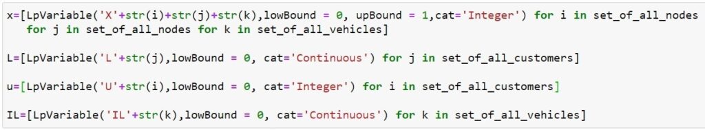
Decision variables
- xkij – Binary variable, 1 if vehicle k travels from node I to node j, 0 otherwise
- Lj: load of vehicle after having serviced customer j
- uj: A variable required to eliminate sub-tours
- ILk: Load of vehicle when leaving the depot
Constraints, Equations, and python code:
- Declaring the decision variables and problem graph
- Constraint to ensure is visited by exactly one vehicle. Relaxing this constraint will allow you to enable a customer to be visited by multiple vehicles


- Flow Conservation Constraint


- Constraint to ensure that the vehicle starts and ends its route at the same prescribed depot


- Constraint to ensure that vehicles does not travel between two depots. We can neglect this constraint if the business needs demand so


- Ensure that the total duration of the vehicle including the service time does not exceed the prescribed time limit


- Sub-tour elimination constraint. Where m is the number of depots and n is the number of customers


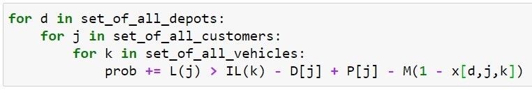
- Vehicle load calculation constraint after the first visit

- Vehicle load calculation constraint after subsequent visits


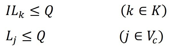
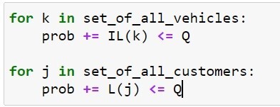
- Constraints to ensure the vehicle load carrying capacity is not violated at any section of the route
Once you have the constraints and decision variables in place, you can then declare an objective function based on minimization of the cost.
Some Advanced Considerations
What will happen if the number of depots, customers, products to be delivered are huge? The size of the linear program would explode and it would be difficult to handle such huge problems using a simple linear programming model. Advanced algorithms like heuristics and a combination of clustering and linear program can be experimented with to arrive to optimal solutions, but the solution may not be the best solution. That is a trade-off to be taken into account for higher solve time and exactness of the model.
Conclusion
As we have just declared a very simple problem, but these constraints can serve as the skeleton for a general framework wherein more complicated constraints can be added as discussed and based on your business problems and make it realistic to tackle any problem that can be faced. This shows the power of mathematical optimization in real life.
Conclusion
https://onlinelibrary.wiley.com/doi/10.1111/itor.12560
Multi-Depots Vehicle Routing Problem with Simultaneous Delivery and Pickup and Inventory Restrictions: Formulation and Resolution – Bouanane et al
Vehicle Routing – Philip Kilby and Paul shaw
A REAL-WORLD CASE STUDY OF A VEHICLE ROUTING PROBLEM UNDER UNCERTAIN DEMAND – Anan Mungwattan et al